BTPS Calculator
Spirometry test is a procedure that measures lung volumes and air flow parameters which calculate from inspiratory and expiratory gas volumes of a human subject.
The gas volumes/flows obtained by the spirometer are in ATPS (Ambient Temperature and Pressure Saturated) conditions which its volumes also depends on environmental conditions including room temperature.
The obtained volumes/flows must be converted to gas condition in BTPS (Body Temperature, Pressure, water vapor Saturated) which gives more accurate representation of actual volumes/flows within the lungs.
BTPS correction factor is a coefficient used to convert flow and volume measured at ambient conditions (ATPS) to the conditions within the lungs (BTPS).
get_btps_factor() is a function to obtain the BTPS correction factor.
# BTPS correction factor at room temperature = 27 degree celsius
btps_factor27 <- get_btps_factor(temp = 27)
btps_factor27
#> [1] 1.063
If Tidal Volume (TV) was measured as 500 ml at room temperature of 27 degree celsius, the TV in the lung at BTPS (body temperature, pressure, water vapor saturated) would be:
# TV (ml) at BTPS
500 * btps_factor27
#> [1] 531.5
If you want to convert several lung volumes or flow (from ATPS to BTPS), use lung_vol_atps_btps() and the result will be shown as a tibble.
lung_vol_atps_btps(
  temp = 27,
  FEV1 = 3.5,
  FVC = 4.5,
  PEF = 450,
  TV = 0.5,
  IC = 2.5,
  EC = 2.5,
  VC = 4.5
)
#> # A tibble: 10 × 4
#>    Parameter  ATPS    BTPS Unit
#>    <chr>     <dbl>   <dbl> <chr>
#>  1 FEV1        3.5   3.72  L
#>  2 FVC         4.5   4.78  L
#>  3 FEV1/FVC   77.8  82.7   %
#>  4 PEF       450   478.    L/min
#>  5 TV          0.5   0.532 L
#>  6 IC          2.5   2.66  L
#>  7 IRV         2     2.13  L
#>  8 EC          2.5   2.66  L
#>  9 ERV         2     2.13  L
#> 10 VC          4.5   4.78  L
Metabolic Rate & Oxygen Consumption Calculator
In a laboratory experiment using Harvard Spirometer, this package provides functions to calculate metabolic rate and oxygen consumption by input a displacement in x-and y-direction of Harvard spirometer tracing, height and weight of the subject, and environmental conditions which are temperature and barometric pressure.
Oxygen Consumption
In Harvard spirometer tracing, horizontal direction (x-direction) represents time (default paper speed = 25 mm/min) whereas vertical direction (y-direction) represents usage of oxygen (1 mm = 30 ml of oxygen). With a little bit of calculation, we can derived an oxygen consumption in unit of L/hr in the ATPS condition (Ambient Temperature and barometric Pressure Saturated with water vapor condition).
You can use get_oxycons() to calculate oxygen consumption and it will also provide other info printed to R console as well.
oxycons <- get_oxycons(x = 15, # displacement in x-direction = 15 mm
            y = 80, # displacement in y-direction = 80 mm
            paper_speed = 25 # Paper speed of the kymograph = 25 mm/min
            )
#> Harvard spirometer tracing:
#>  - Paper speed = 25 mm/min
#>  - Time interval = 0.6 min (horizontal displacement = 15 mm)
#>  - Volume change = 2400 ml (vertical displacement = 80 mm)
#>
#> Oxygen Consumption at ATPS = 240 L/hr
Metabolic Rate
To calculate metabolic rate, we must first convert oxygen consumption \(\dot{V}_{o_2}\) at ATPS to STPD (Standard Temperature of 0°C and a barometric Pressure of 760 mmHg, and in a Dry state).
STPD correction factor can be used to convert gas in ATPS to BTPS condition. It has a linear relationship with barometric pressure and temperature.
Therefore, get_STPD_factor() can be used to predict STPD factor using baro and temp_c as predictors. (It use multiple linear regression model behind the scene.)
stpd_760_25 <- get_STPD_factor(
  baro = 760, # Barometric pressure at the recording site.
  temp_c = 25 # Temperature in celsius at the recording site.
  )
#> STPD correction factor = 0.883 (760 mmHg, 25 degree celcius)
Correction can be made by multiply oxygen consumption \(\dot{V}_{o_2}\) at ATPS to STPD correction factor.
oxycons * stpd_760_25 # Unit in L/hr
#> [1] 211.9386
Finally, metabolic rate can be calculated by times an oxygen consumption \(\dot{V}_{o_2}\) (L/hr) at STPD to a caloric equivalent of oxygen (Cal/hr) divided by Body Surface Area (BSA) in m2, which can be calculated by DuBois & DuBois formula (DuBois D, DuBois EF)
\[
Met \ Rate \ (Cal/m^2/hr) = \frac{ \dot{V}_{o_2} (L/hr) \times CalEqi \ O_2 \ (Cal/hr)}{ BSA \ (m^2) }
\]
get_metabolic_rate() is a final wrapper function that calculate metabolic rate; moreover, it also reports metabolic rate along with oxygen consumption and other related parameters printed to the R console.
get_metabolic_rate(x = 15, # displacement in x-direction = 15 mm
                   y = 80, # displacement in y-direction = 80 mm
                   paper_speed = 25, # Paper speed of the kymograph = 25 mm/min
                   baro = 760, # Barometric pressure at the recording site.
                   temp_c = 25, # Temperature in celsius at the recording site.
                   wt_kg = 70, # Subject's weight in kilogram
                   ht_cm = 180, # Subject's height in centimetre
                   cal_eqi_oxygen = 4.825 # Caloric equivalent of Oxygen at RQ = 0.82
)
#> Harvard spirometer tracing:
#>  - Paper speed = 25 mm/min
#>  - Time interval = 0.6 min (horizontal displacement = 15 mm)
#>  - Volume change = 2400 ml (vertical displacement = 80 mm)
#>
#> Oxygen Consumption at ATPS = 240 L/hr
#>
#> Metabolic rate calculation:
#>  - STPD correction factor = 0.883 (760 mmHg, 25 degree celcius)
#>  - Oxygen Consumption at STPD = 211.939 L/hr (0.883 x 240 L/hr)
#>  - Caloric equivalent of Oxygen = 4.825 Cal/L of Oxygen
#>  - BSA = 1.886 square metre (wt = 70 kg, ht = 180 cm)
#>
#> Metabolic Rate = 542.128 Cal/m2/hr
#>
#>
Simulation of Harvard Spirometer Tracing
Simulate Data
In this section, contrary to the previous, we will simulate data to plot Harvard spirometer tracing from the respiratory parameters.
sim_Harvard_tracing() is the function to simulates volume-time tracing data produced by breathing of a hypothetical subject as recorded by the Harvard spirometer.
The input parameters can be categorized into the followings:
Function to Simulate 1 Respiratory Cycle: as supply by the argument
f, the default, currently, is a cosine (cos) function which might give a rough representation of 1 respiratory cycle. (It is not a physiologic representation of respiratory waveform. I still need more research on this.)Amplitude and Wavelength of the sinusoidal function: this can be calculated by knowing the Respiratory Rate (
RR), Tidal Volume (TV), and paper speed (paper_speed)-
Slope and Y-intercept of an Oxygen Line: the oxygen line, i.e., the linear line fitted from the lowest points of each respiratory waveform, can be simulated by knowing its slope (\(\beta_1\)), y-intercept (\(\beta_0\)), and random error term (\(\epsilon\)).
-
Slope (\(\beta_1\)) can be calculated from an oxygen consumption (argument
oxycons) and paper speed (paper_speed). - Y-intercept (\(\beta_0\)) can be specified directly from the user.
- And, a random error (\(\epsilon\)) can be generated from a Gaussian distribution with \(\mu\) = 0, and
sdas specified.
-
Slope (\(\beta_1\)) can be calculated from an oxygen consumption (argument
tracing_df <- sim_Harvard_tracing(
  f = "cos",         # Cosine function to represent 1 respiratory cycle
  t_start = 0,       # First `x` value will be started at time = 0 minute
  t_end = 1,         # Last `x` value will be ended at time = 1 minute
  paper_speed = 25,  # Paper speed in mm/minute
  y_int_O2_line = 5, # Y-intercept of an oxygen line
  oxycons = 10,      # Oxygen consumption is 10 L/hr (default unit)
  TV = 500,          # Tidal Volume is 500 ml
  RR = 20,           # Respiratory Rate is 20 /min
  seq_x_by = 0.01,   # This control resolution of simulated data
  epsilon_sd = 0.3,  # Add random variation sampled from Gaussian distribution with mean = 0, sd = 0.3
  seed = 1,          # Seed to generate the random variation
)

head(tracing_df)
#>      x        y y_O2_line
#> 1 0.00 4.812064  4.812064
#> 2 0.01 5.067841  5.057315
#> 3 0.02 4.795831  4.753756
#> 4 0.03 5.579820  5.485251
#> 5 0.04 5.275616  5.107741
#> 6 0.05 5.026778  4.764971
Plot
With a little help of ggplot2 package, the tracing can then be visualized.
ggplot(tracing_df) +
  geom_path(aes(x, y)) +
  geom_smooth(aes(x, y_O2_line), method = "lm", formula = "y~x",
              linetype = "dashed") +
  expand_limits(y = 0) +
  labs(title = "Simulation of Harvard Spirometer Tracing",
        subtitle = TeX("(TV = 500 ml, RR = 20/min, $\\dot{V}_{O_2}$ = 10 L/hr)"),
        x = "x (mm)", y = "y (mm)")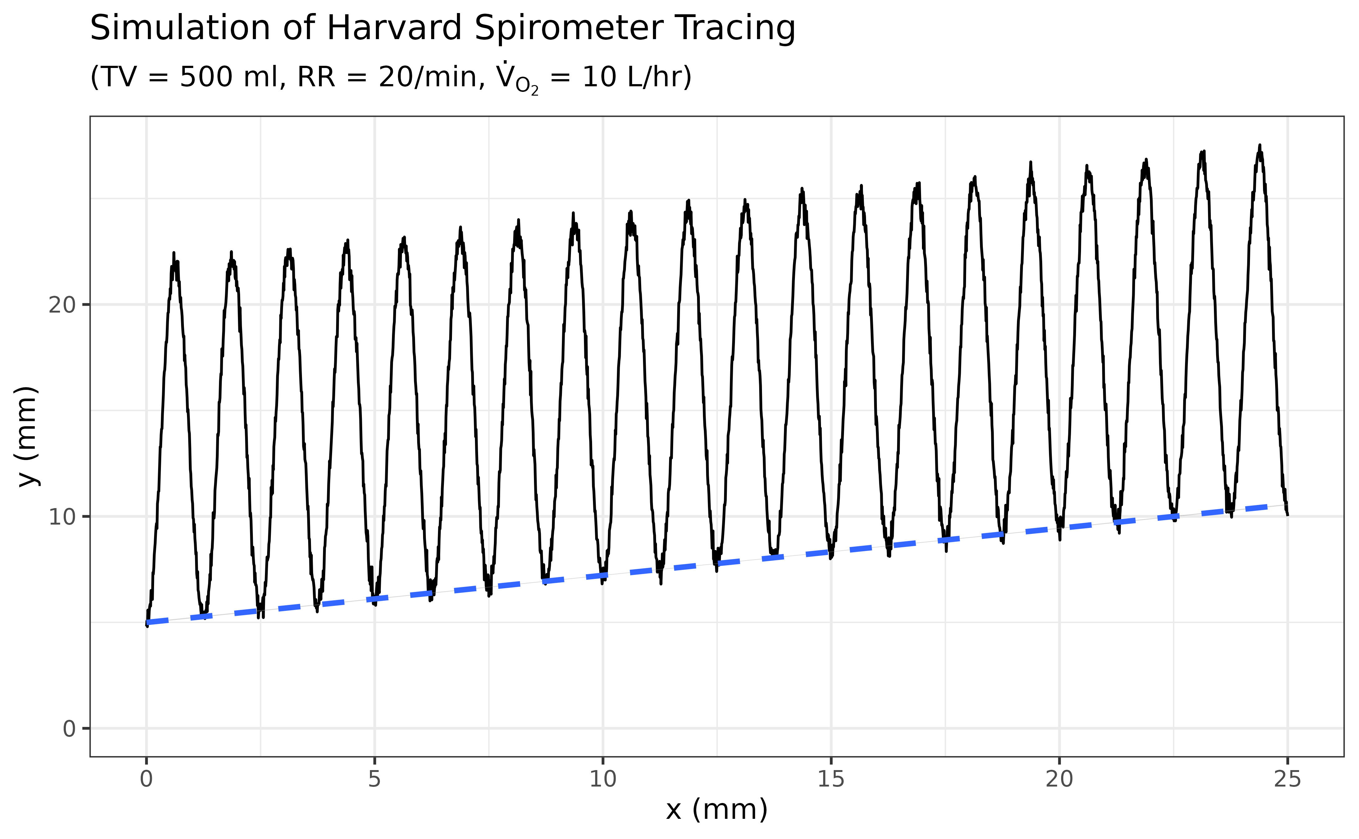
Behind the Tracing
If you curious about the mathematical model that underlies this simulated tracing, please visit this article.